# No more business as usual - Agile and effective responses to emerging pathogen threats require open data and open analytics

(opens new window)

This repo serves as a companion to our study describing the analysis of early COVID-19 data:

No more business as usual: agile and effective responses to emerging pathogen threats require open data and open analytics (opens new window). usegalaxy.org, usegalaxy.eu, usegalaxy.org.au, usegalaxy.be and hyphy.org development teams, Anton Nekrutenko, Sergei L Kosakovsky Pond. Plos-Pathogens August 13, 2020; doi: https://doi.org/10.1371/journal.ppat.1008643

It contains descriptions of workflows and exact versions of all software used. The goals of this study were to:

Underscore the importance of access to raw data
Demonstrate that existing community efforts in curation and deployment of biomedical software can reliably support rapid reproducible research during global crises

Our analysis was divided into six parts listed below (we also added "Updates" section where will be keeping track of new data as it appears). Each part has a dedicated page that provides links to input datasets, intermediate and final results, workflows, and Galaxy histories that list all details for each analysis. These workflows can be re-run by any of three global Galaxy instances in the US (opens new window), in Europe (opens new window) and in Australia (opens new window), as well as in the ELIXIR Belgium (opens new window) Galaxy instance. NOTE: if you are analysing data generated using the ARTIC sequencing protocol look at the ARTIC page.

In addition we will be looking at newly released data here → Updates: Analysis of additional data

The analyses have been performed using the Galaxy (opens new window) platform and open source tools from BioConda (opens new window). Tool runs used XSEDE (opens new window) resources maintained by the Texas Advanced Computing Center ( TACC (opens new window)), Pittsburgh Supercomputing Center (PSC (opens new window)), and Indiana University (opens new window) in the U.S., de.NBI (opens new window) and VSC (opens new window) cloud resources on the European side, and ARDC (opens new window) cloud resources in Australia.

# Pre-processing

# Preprocessing of raw SARS-CoV-2 reads

The raw reads available so far are generated from bronchoalveolar lavage fluid (BALF) and are metagenomic in nature: they contain human reads, reads from potential bacterial co-infections as well as true COVID-19 reads.

# Live Resources

usegalaxy.org	usegalaxy.eu	usegalaxy.org.au	usegalaxy.be	usegalaxy.fr

# What's the point?

Assess quality of reads, remove adapters and remove reads mapping to human genome.

# The outline

Illumina and Oxford nanopore reads are pulled from the NCBI SRA (links to SRA accessions are available here (opens new window)). They are then processed separately as described in the workflow section.

# Inputs

💥 If you experience problems downloading data from NCBI SRA, use Galaxy history pre-populated with inputs as described in "Alternate Workflow" section below.

Only SRA accessions are required for this analysis. The described analysis was performed with all SRA SARS-CoV accessions available as of Feb 20, 2020:

Illumina reads
```
SRR10903401
SRR10903402
SRR10971381
```
Oxford Nanopore reads
```
SRR10948550
SRR10948474
SRR10902284
```

# Outputs

This workflow produces three outputs that are used in two subsequent analyses:

#	Output	Used in
1.	A combined set of adapter-free Illumina reads without human contamination	Assembly
2.	A combined set of Oxford Nanopore reads without human contamination	Assembly
3.	A collection of adapter-free Illumina reads from which human reads have not been removed	Variation detection

# The history and the workflow

A Galaxy workspace (history) containing the most current analysis can be imported from here (opens new window).

The publicly accessible workflow (opens new window) can be downloaded and installed on any Galaxy instance. It contains version information for all tools used in this analysis.

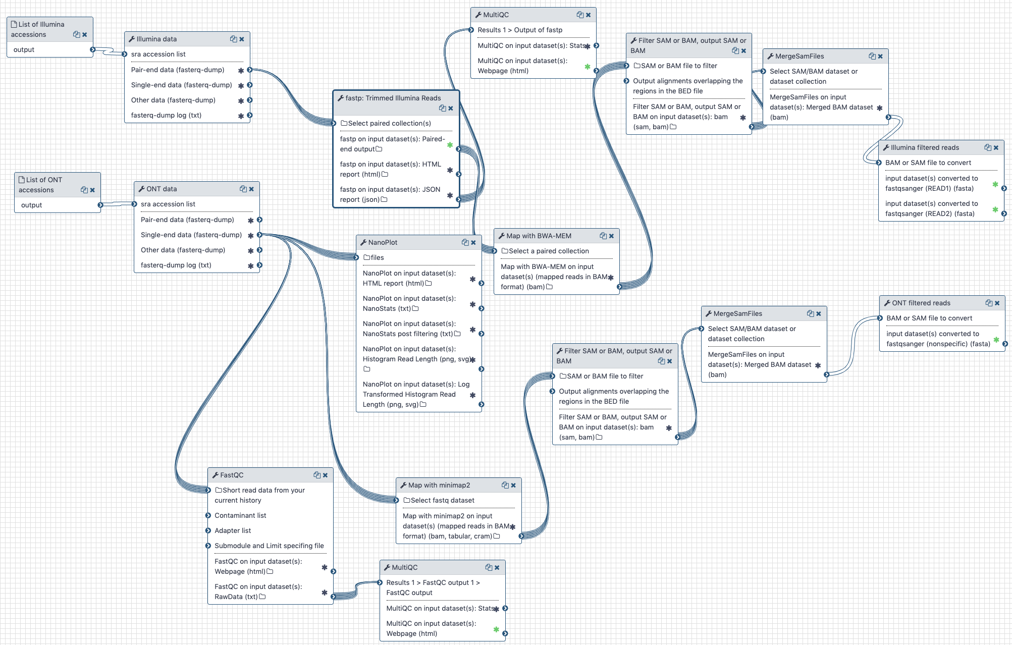
The workflow performs the following steps:

# Illumina

Illumina reads are QC'ed and adapter sequences are removed using fastp
Quality metrics are computed and visualized using fastqc and multiqc
Reads are mapped against human genome version hg38 using bwa mem
Reads that do not map to hg38 are filtered out using samtools view
Reads are converted back to fastq format using samtools fastx

# Oxford nanopore

Reads are QC'ed using nanoplot
Quality metrics are computed and visualized using fastqc and multiqc
Reads are mapped against human genome version hg38 using minimap2
Reads that do not map to hg38 are filtered out using samtools view
Reads are converted back to fastq format using samtools fastx

# BioConda

Tools used in this analysis are also available from BioConda:

Name	Link
`sra-tools`	(opens new window)
`fastqc`	(opens new window)
`multiqc`	(opens new window)
`fastp`	(opens new window)
`nanoplot`	(opens new window)
`bwa`	(opens new window)
`picard`	(opens new window)
`samtools`	(opens new window)

# Alternate Workflow

An alternate starting point has been created for those not wanting to wait for the data to be downloaded from the NCBI SRA. (This can especially be an issue in Australia or Europe.)

There is a shared history (opens new window) containing all of the starting data in appropriate collections and an alternate workflow (opens new window) able to make use of this alternate input. Apart from a slightly different starting point, the workflow and the outputs it produces are identical to that above.

usegalaxy.org	usegalaxy.eu	usegalaxy.org.au	usegalaxy.be

# Assembly

# Assembly of SARS-CoV-2 from pre-processed reads

# Live Resources

usegalaxy.org	usegalaxy.eu	usegalaxy.org.au	usegalaxy.be	usegalaxy.fr

# What's the point?

Use a combination of Illumina and Oxford Nanopore reads to produce SARS-CoV-2 genome assembly.

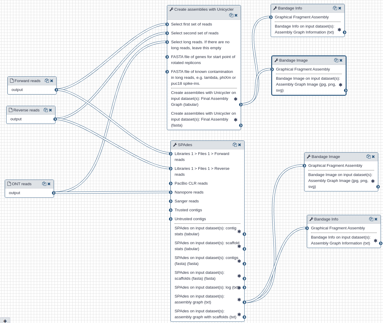
# Outline

We use Illumina and Oxford Nanopore reads that were pre-processed to remove human-derived sequences. We use two assembly tools: spades (opens new window) and unicycler (opens new window). While spades is a tool fully dedicated to assembly, unicycler is a "wrapper" that combines multiple existing tools. It uses spades as an engine for short read assembly while utilizing mimiasm (opens new window) and racon (opens new window) for assembly of long noisy reads.

In addition to assemblies (actual sequences) the two tools produce assembly graphs that can be used for visualization of assembly with bandage (opens new window).

# Inputs

Filtered Illumina and Oxford Nanopore reads produced during the pre-processing step are used as inputs to the assembly tools.

# Outputs

Each tool produces assembly (contigs) and assembly graph representations. The largest contigs generated by unicycler and spades were 29,781 and 29,907 nts, respectively, and had 100% identity over their entire length.

The following figures show visualizations of assembly graphs produced with spades and unicycler. The complexity of the graphs is not surprising given the metagenomic nature of the underlying samples.

Assembly graphs for Unicycler (A) and SPAdes (B)

A. Unicycler assembly graph

B. SPAdes assembly graph

# History and workflow

A Galaxy workspace (history) containing the most current analysis can be imported from here (opens new window).

The publicly accessible workflow (opens new window) can be downloaded and installed on any Galaxy instance. It contains version information for all tools used in this analysis.

# BioConda

Tools used in this analysis are also available from BioConda:

Name	Link
`unicycler`	(opens new window)
`spades`	(opens new window)
`bandage`	(opens new window)

# MRCA

# Dating the most recent common ancestor (MRCA) of SARS-CoV-2

# Live Resources

usegalaxy.org	usegalaxy.eu	usegalaxy.org.au	usegalaxy.be	usegalaxy.fr

# What's the point?

To estimate the time of COVID-19 emergence we use simple root-to-tip regression (Korber et al. 2000 (opens new window); more complex and powerful phylodynamics methods could certainly be used, but for this data with very low levels of sequence divergence, simpler and faster methods suffice). From the set of all COVID-19 sequences available as of Feb 16, 2020 we obtain an MRCA date of Oct 24, 2019, which is close to other existing estimates Rambaut 2020 (opens new window).

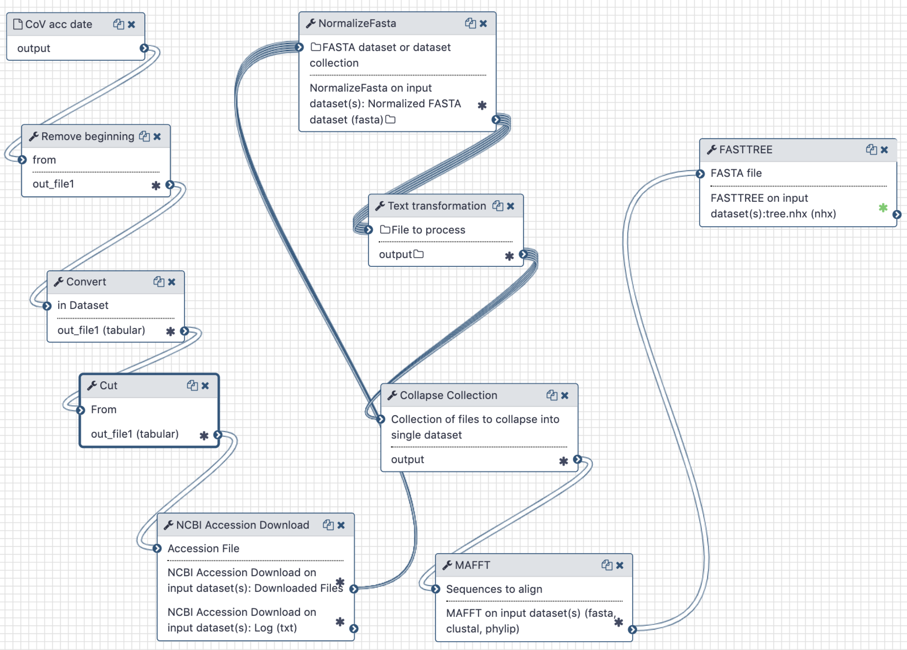
# Outline

This analysis consists of two components - a Galaxy workflow and a Jupyter notebook. To use a Jupyter Notebook in a Galaxy workflow see these short instructions (opens new window).

The workflow is used to extract full length sequences of SARS-CoV-2, tidy up their names in FASTA files, produce a multiple sequences alignment and compute a maximum likelihood tree.

The Jupyter notebook is used to correlate branch lengths with collection dates in order to estimate MRCA timing.

# Inputs

One input is required: a comma-separated file containing accession numbers and collection dates:

Accession,Collection_Date
MT019531,2019-12-30
MT019529,2019-12-23
MT007544,2020-01-25
MN975262,2020-01-11
...

An up-to-date version of this file can be generated directly from the NCBI Virus (opens new window) resource by

searching for SARS-CoV-2 (NCBI taxid: 2697049) sequences
configuring the list of results to display only the Accession and Collection date columns
downloading the Current table view result in CSV format

The collection dates will be taken from the corresponding GenBank record's /collection_date tag.

# Outputs

The Galaxy workflow generates a maximum-likelihood phylogenetic tree. This tree and the initial workflow input of accession numbers and collection times are then used in the Jupyter notebook to calculate an estimate of the time to the most recent common ancestor of all samples.

# History and workflow

A Galaxy workspace (history) containing the most current analysis can be imported from here (opens new window).

The publicly accessible workflow (opens new window) can be downloaded and installed on any Galaxy instance. It contains version information for all tools used in this analysis.

# BioConda

Tools used in this analysis are also available from BioConda:

Name	Link
`ncbi-acc-download`	(opens new window)
`picard`	(opens new window)
`mafft`	(opens new window)
`fasttree`	(opens new window)

# Variation

# Analysis of variation within individual COVID-19 samples | 🔥 updated weekly

Last update = May 20

# Live Resources

usegalaxy.org	usegalaxy.eu	usegalaxy.org.au	usegalaxy.be	usegalaxy.fr

# What's the point?

The absolute majority of SARS-COV-2 data is in the form of assembled genomic sequences. This is unfortunate because any variation that exists within individual samples is obliterated--converted to the most frequent base--during the assembly process. However, knowing underlying evolutionary dynamics is critical for tracing evolution of the virus as it allows identification of genomic regions under different selective regimes and understanding of its population parameters.

# Outline

In this analysis we check for new data, run single- or paired-end analysis workflows, aggregate the results, combine them with the list produced in the previous days, and finally analyze the complete, up-to-date set of variants using Jupyter. Here is a brief outline with links:

Step	Description
Obtain Illumina read accessions	Generate list of newly released Illumina datasets. Performed daily.
(opens new window)	If data is paired-end → run PE workflow
(opens new window)	If data is single-end → run SE workflow
(opens new window)	Combine results of PE and SE workflow. This is done in a single Galaxy history that is used to aggregate results of all daily runs.
(opens new window)	Start Jupyter notebook to analyze variants (it can started directly from history linked at the previous step)

# Obtaining the data

Raw sequencing reads are required to detection of within-sample sequence variants. We update the list of available data daily using the following logic implemented in fetch_sra_acc.sh:

Fetch accessions from SARS-CoV-2 resource (opens new window), Short Read Archive at NCBI (opens new window), and EBI (opens new window). This is done daily.
A union of accessions from these three resources is then computed (union.txt).
Sample metadata is then obtained for all retained accession numbers and saved into current_metadata.txt.
Metadata is used to split datasets into current_illumina.txt and current_gridion.txt.
In addition, we fetch all publicly available complete SARS-CoV-2 genomes. These are stored in genome_accessions.txt and current_complete_ncov_genomes.fasta.

The list of currently analyzed datasets (as of April 28, 2020) is shown in Table 1 below.

Table 1. SARS-CoV-2 Illumina datasets and corresponding analysis histories.

Date	Galaxy history
Beginning of outbreak - March 20, 2020	Paired End (opens new window) Single End (opens new window)
March 25, 2020	Paired and Single Ends (opens new window)
March 26, 2020	Paired End (opens new window)
April 2, 2020	Paired and Single Ends (opens new window)
April 8, 2020	Paired and Single Ends (opens new window)
April 28, 2020	Paired and Single Ends (opens new window)
May 2, 2020	Paired and Single Ends (opens new window)
May 9, 2020	Paired and Single Ends (opens new window)
May 17, 2020	Paired and Single Ends (opens new window)
May 18, 2020	Paired and Single Ends (opens new window)
History for aggregation	(https://usegalaxy.org/u/sars-cov2-bot/h/covid19-variant-aggregation-analysis)

# How do we call variants?

This section provides background of how we settled on using lofreq as the principal variant caller for this project.

# Calling variants in haploid mixtures is not standardized

The development of modern genomic tools and formats have been driven by large collaborative initiatives such as 1,000 Genomes, GTEx and others. As a result the majority of current variant callers have been originally designed for diploid genomes of human or model organisms where discrete allele frequencies are expected. Bacterial and viral samples are fundamentally different. They are represented by mixtures of multiple haploid genomes where the frequencies of individual variants are continuous. This renders many existing variant calling tools unsuitable for microbial and viral studies unless one is looking for fixed variants. However, recent advances in cancer genomics have prompted developments of somatic variant calling approaches that do not require normal ploidy assumptions and can be used for analysis of samples with chromosomal malformations or circulating tumor cells. The latter situation is essentially identical to viral or bacterial resequencing scenarios. As a result of these developments the current set of variant callers appropriate for microbial studies includes updated versions of “legacy” tools (FreeBayes (opens new window) and mutect2 (a part of GATK (opens new window)) as well as dedicated packages (Breseq (opens new window), SNVer (opens new window), and lofreq (opens new window)). To assess the applicability of these tools we first considered factors related to their long-term sustainability, such as the health of the codebase as indicated by the number of code commits, contributors and releases as well as the number of citations. After initial testing we settled on three callers: FreeBayes, mutect2, and lofreq (Breseq’s new “polymorphism mode” has been in experimental state at the time of testing. SNVer is no longer actively maintained). FreeBayes contains a mode specifically designed for finding sites with continuous allele frequencies; Mutect2 features a so called mitochondrial mode, and lofreq was specifically designed for microbial sequence analysis.

# Benchmarking callers: `lofreq` is the best choice

Our goal was to identify variants in mixtures of multiple haplotypes sequenced at very high coverage. Such dataset are typical in modern bacterial and viral genomic studies. In addition, we are seeking to be able to detect variants with frequencies around the NGS detection threshold of ~ 1% (Salk et al. 2018 (opens new window)). In order to achieve this goal we selected a test dataset, which is distinct from data used in recent method comparisons (Bush et al. 2019 (opens new window); Yoshimura et al. 2019 (opens new window)). These data originate from a duplex sequencing experiment recently performed by our group (Mei et al. 2019 (opens new window)). In this dataset a population of E. coli cells transformed with pBR322 plasmid is maintained in a turbidostat culture for an extensive period of time. Adaptive changes accumulated within the plasmid are then revealed with duplex sequencing (Schmitt et al. 2012 (opens new window)). Duplex sequencing allows identification of variants at very low frequencies. This is achieved by first tagging both ends of DNA fragments to be sequenced with unique barcodes and subjecting them to paired-end sequencing. After sequencing read pairs containing identical barcodes are assembled into families. This procedure allows to reliably separate errors introduced during library preparation and/or sequencing (present in some but not all members of a read family) from true variants (present in all members of a read family derived from both strands).

For the following analysis we selected two data points from Mei et al. 2019 (opens new window): one corresponding to the beginning of the experiment (s0) and the other to the end (s5). The first sample is expected to be nearly clonal with no variation, while the latter contains a number of adaptive changes with frequencies around 1%. We aligned duplex consensus sequences (DCS) against the pBR322. We then walked through read alignments to produce counts of non-reference bases at each position (Fig. 1).

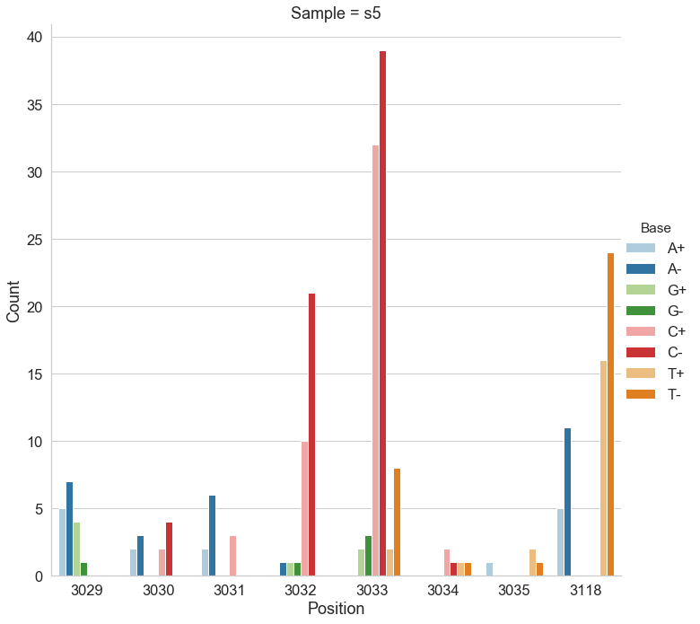
Figure 1. Counts of alternative bases at eight variable locations within pBR322.

Because all differences identified this way are derived from DCS reads they are a reasonable approximation for a “true” set of variants. s0 and s5 contained 38 and 78 variable sites with at least two alternative counts, respectively (among 4,361 bases on pBR322) of which 27 were shared. We then turned our attention to the set of sites that were determined by Mei et al. to be under positive selection (sites 3,029, 3,030, 3,031, 3,032, 3,033, 3,034, 3,035, 3,118). Changes at these sites increase the number of plasmid genomes per cell. Sample s0 does not contain alternative bases at any of these sites. Results of the application of the three variant callers with different parameter settings (shown in Table 2) are summarized in Fig. 2.

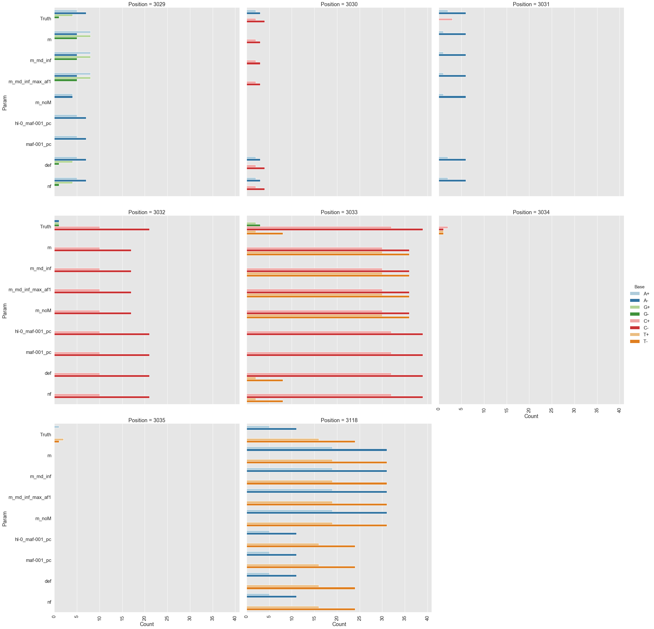
Figure 2. Calls made by mutect2, freebayes, and lofreq. For explanation of x-axis labels see Table 2.

The lofreq performed the best followed by mutect2 and FreeBayes (contrast "Truth" with "nf" and "def" in Fig. 2). The main disadvantage of mutect2 is in its handling of multiallelic sites (e.g., 3,033 and 3,118) where multiple alternative bases exist. At these sites mutect2 outputs alternative counts for only one of the variants (the one with highest counts; this is why at site 3,118 A and T counts are identical). Given these results we decided to use lofreq for the main analysis of the data.

Table 2. Command line options for each caller.

Caller	Command line	Figure 2 label
`mutect2`	`--mitochondria-mode true`	m
`mutect2`	default	m_noM
`mutect2`	`--mitochondria-mode true --f1r2-max-depth 1000000`	m_md_inf
`mutect2`	`--mitochondria-mode true --f1r2-max-depth 1000000 -max-af 1`	m_md_inf_max_af1
`freebayes`	`--haplotype-length 0 --min-alternate-fraction 0.001 --min-alternate-count 1 --pooled-continuous --ploidy 1`	hl-0_maf-001_pc
`freebayes`	`-min-alternate-fraction 0.001 --pooled-continuous --ploidy 1`	maf-001_pc
`lofreq`	`--no-default-filter`	nf
`lofreq`	default	def

# Galaxy workflows

lofreq is used in two galaxy workflows described in this section. Illumina data currently available for SARS-CoV-2 consists of paired- and single-end datasets. We use two similar yet distinct workflows to analysis these datasets.

# Analysis of Illumina Paired End data

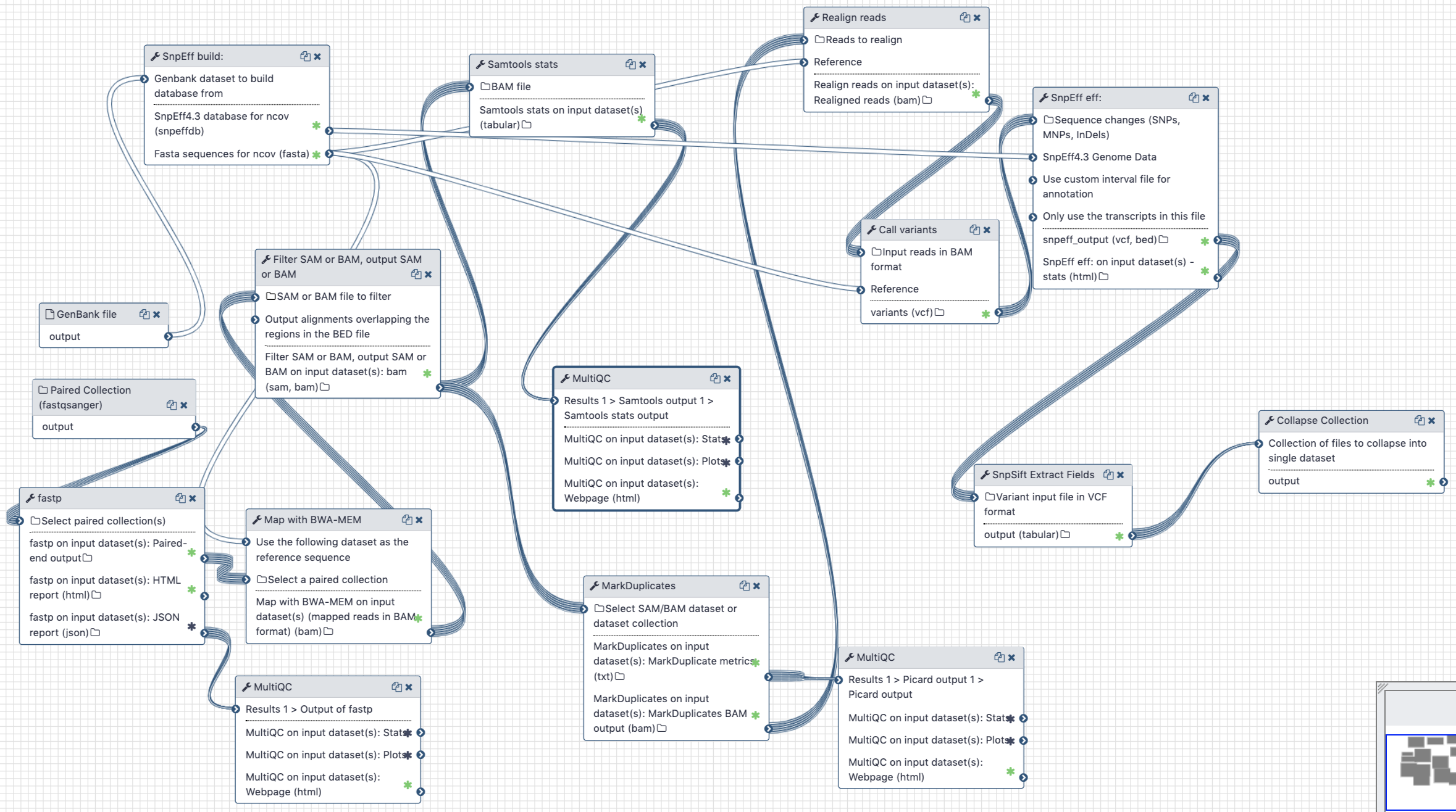
Figure 3. Workflow for the analysis of paired-end Illumina reads (opens new window)

# Inputs:

GenBank file for the reference COVID-19 genome (opens new window). The GenBank record is used by snpeff to generate a database for variant annotation.
Downloaded paired-end reads in fastq format as a paired dataset collection. Reads can be downloaded using Galaxy's wrapper for fasterq-dump located in "Get data" tool section.

# Steps:

Map all reads against COVID-19 reference NC_045512.2 (opens new window) using bwa mem
Filter reads with mapping quality of at least 20, that were mapped as proper pairs
Mark duplicate reads with picard markduplicates
Perform realignments using lofreq viterbi
Call variants using lofreq call
Annotate variants using snpeff against database created from NC_045512.2 GenBank file
Convert VCFs into tab delimited dataset

# Outputs

A tab-delimited table of variants described in Table 2 below.

# Analysis of Illumina Single End data

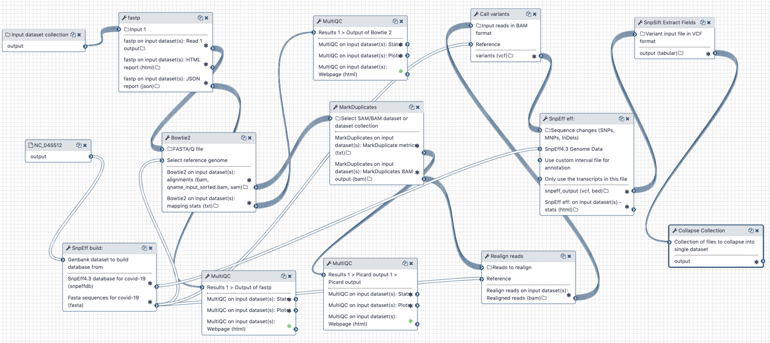Figure 4. Workflow for the analysis of single-end Illumina reads < 100 bp (opens new window)

# Inputs:

GenBank file for the reference COVID-19 genome (opens new window). The GenBank record is used by snpeff to generate a database for variant annotation.
Downloaded paired-end reads in fastq format as a dataset collection. Reads can be downloaded using Galaxy's wrapper for fasterq-dump located in "Get data" tool section.

# Steps:

Map all reads against COVID-19 reference NC_045512.2 (opens new window) using bowtie2 (because all SE datasets we have seen so far contain short, 75 bp, reads)
Filter reads with mapping quality of at least 20
Mark duplicate reads with picard markduplicates
Perform realignments using lofreq viterbi
Call variants using lofreq call
Annotate variants using snpeff against database created from NC_045512.2 GenBank file
Convert VCFs into tab delimited dataset

# Output

After running both workflows the data is combined into a single dataset (variant_list.tsv and smaller dataset filtered at alternative allele frequency of 5% and above variant_list.05.tsv).

These result datasets have the following structure:

Table 3. Output of PE and SE workflows described above. Here, most fields names are descriptive. SB = the Phred-scaled probability of strand bias as calculated by lofreq (opens new window) (0 = no strand bias); DP4 = strand-specific depth for reference and alternate allele observations (Forward reference, reverse reference, forward alternate, reverse alternate).

	Sample	CHROM	POS	REF	ALT	DP	AF	SB	DP4	IMPACT	FUNCLASS	EFFECT	GENE	CODON
0	SRR10903401	NC_045512	1409	C	T	124	0.040323	1	66,53,2,3	MODERATE	MISSENSE	NON_SYNONYMOUS_CODING	orf1ab	Cat/Tat
1	SRR10903401	NC_045512	1821	G	A	95	0.094737	0	49,37,5,4	MODERATE	MISSENSE	NON_SYNONYMOUS_CODING	orf1ab	gGt/gAt
2	SRR10903401	NC_045512	1895	G	A	107	0.037383	0	51,52,2,2	MODERATE	MISSENSE	NON_SYNONYMOUS_CODING	orf1ab	Gta/Ata
3	SRR10903401	NC_045512	2407	G	T	122	0.024590	0	57,62,1,2	MODERATE	MISSENSE	NON_SYNONYMOUS_CODING	orf1ab	aaG/aaT
4	SRR10903401	NC_045512	3379	A	G	121	0.024793	0	56,62,1,2	LOW	SILENT	SYNONYMOUS_CODING	orf1ab	gtA/gtG

# Jupyter notebook

Upon completion of single- and paired-end analysis workflows and combining their results into a single file this file is loaded into a (opens new window). The notebook is used to produce summaries such as distribution of variants across the SARS-CoV-2 genome:

The variants we identified were distributed across the SARS-CoV-2 genome in the following way:

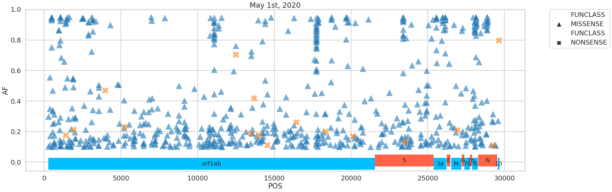
Figure 5. Distribution of variants across the viral genome.

# Galaxy histories

Galaxy histories corresponding to all analyses performed so far are listed in Table 1. The history used for aggregating results and launching jupyter notebook is here → (opens new window).

# BioConda

Tools used in this analysis are also available from BioConda:

Name	Link
`bwa`	(opens new window)
`samtools`	(opens new window)
`lofreq`	(opens new window)
`snpeff`	(opens new window)
`snpsift`	(opens new window)
`porechop`	(opens new window)
`filtlong`	(opens new window)
`minimap2`	(opens new window)
`bowtie2`	(opens new window)

# Annotation

# Functionnal annotation - Example analysis of S-protein polymorphism

# Live Resources

usegalaxy.org	usegalaxy.eu	usegalaxy.org.au	usegalaxy.be	usegalaxy.fr

# What's the point?

In the previous portion (opens new window) of this study, we found variations in SARS-2 Cov genome. To evaluate the impact of variations on the virus, we need to perform functional annotation of variants. A lot of literature is available on a wide variety of species of coronaviruses. To help with that task, we offer two valuable tools :

Tables of coordinate conversion between different species of coronaviruses, to help with the transfer of annotations
Tables of annotation of all residues. Compilated literature on Coronaviruses links each residue to their functional annotation, including from other species of coronavirus.

To illustrate the process, we studied a non-synonymous polymorphism within the S-gene found in the previous portion (opens new window). We are trying to interpret its possible effect.

# Outline

Obtain coding sequences of S proteins from a diverse group of coronaviruses, and generate amino acid alignment to create a table of coordinate conversion.

# Input

Downloaded CDS sequences of coronavirus Spike proteins from NCBI Viral Resource (opens new window) for the following coronaviruses:

Accession	Description
FJ588692.1	Bat SARS Coronavirus Rs806/2006
KR559017.1	Bat SARS-like coronavirus BatCoV/BB9904/BGR/2008
KC881007.1	Bat SARS-like coronavirus WIV1
KT357810.1	MERS coronavirus isolate Riyadh_1175/KSA/2014
KT357811.1	MERS coronavirus isolate Riyadh_1337/KSA/2014
KT357812.1	MERS coronavirus isolate Riyadh_1340/KSA/2014
KF811036.1	MERS coronavirus strain Tunisia-Qatar_2013
AB593383.1	Murine hepatitis virus
AF190406.1	Murine hepatitis virus strain TY
AY687355.1	SARS coronavirus A013
AY687356.1	SARS coronavirus A021
AY687361.1	SARS coronavirus B029
AY687365.1	SARS coronavirus C013
AY687368.1	SARS coronavirus C018
AY648300.1	SARS coronavirus HHS-2004
DQ412594.1	SARS coronavirus isolate CUHKtc10NP
DQ412596.1	SARS coronavirus isolate CUHKtc14NP
DQ412609.1	SARS coronavirus isolate CUHKtc32NP
MN996528.1	SARS-2 Cov
MN996527.1	SARS-2 Cov
NC_045512.2	SARS-2 Cov
NC_002306.3	Feline infectious peritonitis virus
NC_028806.1	Swine enteric coronavirus strain Italy/213306/2009
NC_038861.1	Transmissible gastroenteritis virus

These viruses were chosen based on a publication by Duquerroy et al. (2005 (opens new window)). The sequences were extracted manually--a painful process.

# Output

We produce two alignments, one at the nucleotide and one at the amino acid level, of Betacoronavirus spike proteins. The alignments can be visualized with the Multiple Sequence Alignment Visualization in Galaxy :

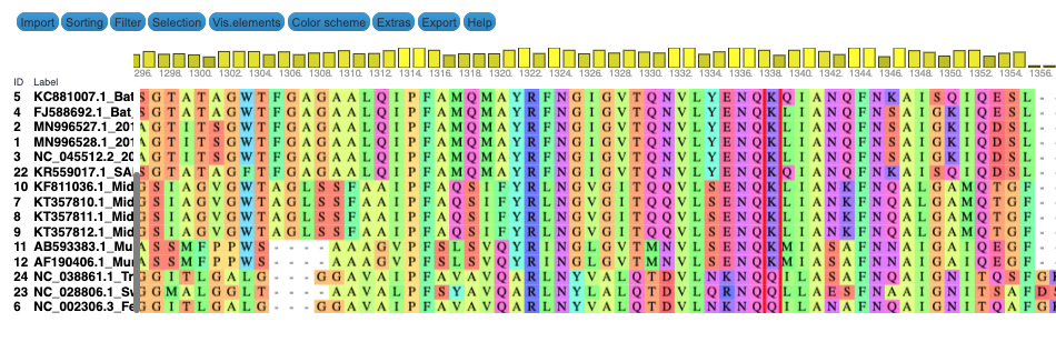
Visualization of amino acid alignment in Galaxy

Alignments of Spike proteins

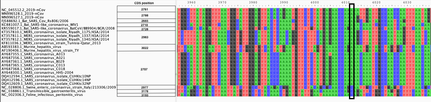A. CDS alignments

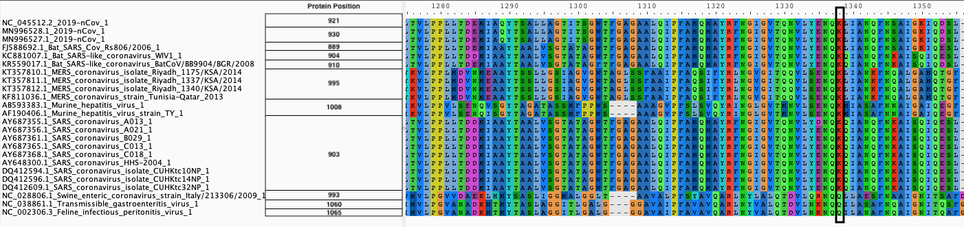B. Protein alignment

# Workflow and history

The Galaxy history containing the latest analysis can be found here (opens new window). The publicly accessible workflow (opens new window) can be downloaded and installed on any Galaxy instance. It contains all information about tool versions and parameters used in this analysis.

Analysis Workflow

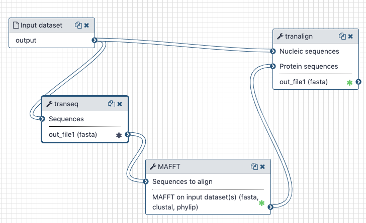
The transeq tool converts the CDS sequences into protein sequences, which we then align with each other using mafft. The output is fed into tranalign along with the nucleotide sequences. tranalign produces a nucleotide alignment coherent with the protein alignment.

# Generation of Coordinate maps

We used this workflow to generate alignment across Coronaviruses for each gene of SARS-2 Cov. From these alignments, using mafft, we created coordinate conversion. The mafft -add option allows the addition of sequences to an alignment, but also generated mapping of the new sequence to the coordinate in the alignment. We reported these mapping data to the SARS-2 Cov coordinate for more clarity.

These tables can be queried through the notebook included in this section. To find positions equivalent to your residue or region of interest :

Select the Gene
Select the species in which your coordinates are
Select the region of interest

# Residue annotations

Since the beginning of this project, we have been compilating functional information from literature for each residue of each gene of SARS-2 cov. The literature covers several species of coronavirus, and we used the coordinate tables presented above to transfer the annotations between species. In cases where the residue is different from the one annotated, it is specified in the table, and all annotations are linked to their article of origin. Due to the considerable amount of literature available, the annotations are incomplete, but we are working on enriching them every day. You can contribute to the annotation effort by adding annotations in the tables on Github (opens new window)

# BioConda

Tools used in this analysis are also available from BioConda:

Name	Link
`mafft`	(opens new window)
`emboss`	(opens new window)

# Notebooks

Source notebook: https://observablehq.com/@delphine-l/coordinate-conversion-between-species-of-coronavirus

Source notebook: https://observablehq.com/@delphine-l/annotation-of-sars-2-coronavirus-genome

# RecombinationSelection

# Evolutionary Analysis

# Live Resources

usegalaxy.org	usegalaxy.eu	usegalaxy.org.au	usegalaxy.be	usegalaxy.fr

# What's the point?

Wu et al. (opens new window) showed recombination between COVID-19 and bat coronaviruses located within the S-gene. We want to confirm this observation and provide a publicly accessible workflow for recombination detection.

In previous coronavirus outbreaks (SARS), retrospective analyses determined that adaptive substitutions might have occurred in the S-protein Zhang et al. (opens new window), e.g., related to ACE2 receptor utilization (opens new window). While data on COVID-19 are currently limited, we investigated whether or not the lineage leading to them showed any evidence of positive diversifying selection.

# Outline

We employ a recombination detection algorithm (GARD) developed by Kosakovsky Pond et al. (opens new window) and implemented in the hyphy package. To select a representative set of S-genes we perform a blast search using the S-gene CDS from NC_045512 (opens new window) as a query against the nr database. We select coding regions corresponding to the S-gene from a number of COVID-19 genomes and original SARS isolates. This set of sequences can be found in this repository

We then generate a codon-based alignment using the workflow shown below and perform the recombination analysis using the gard tool from the hyphy package.

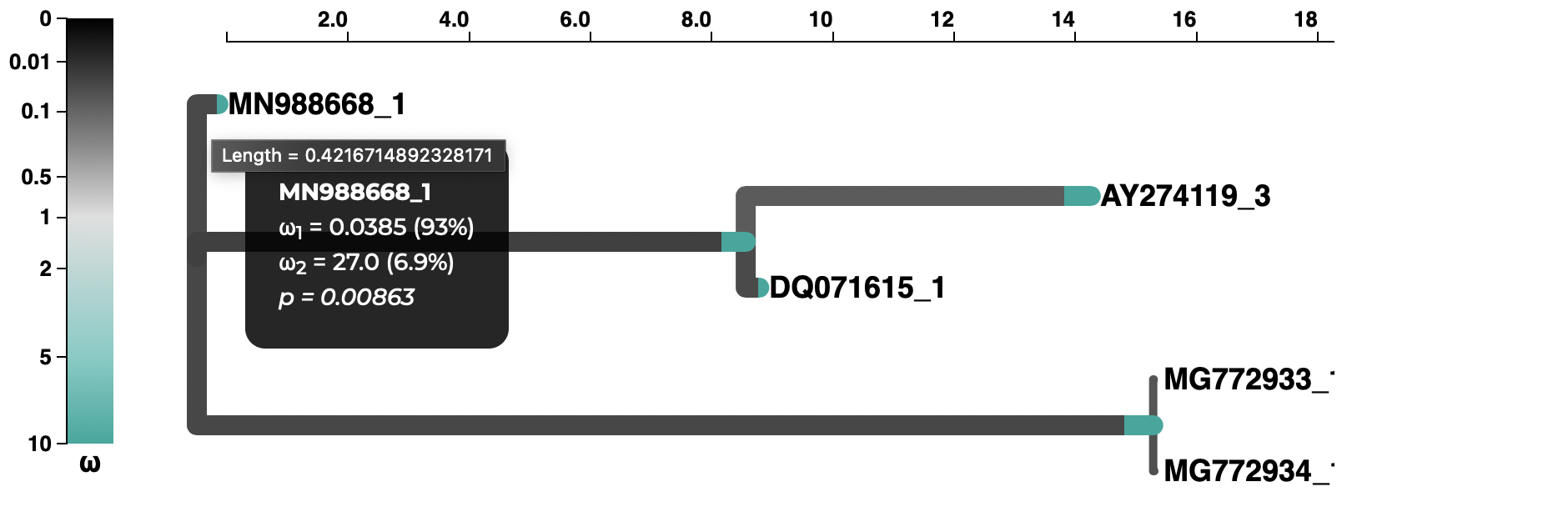
For selection analyses, we apply the Adaptive Branch Site Random Effects (opens new window) method to test whether or each branch of the tree shows evidence of diversifying positive selection along a fraction of sites using the absrel tool from the hyphy package.

# Inputs

A set of unaligned CDS sequences for the S-gene.

# Outputs

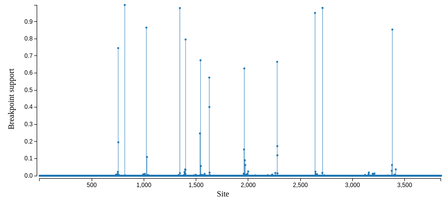
A recombination report:

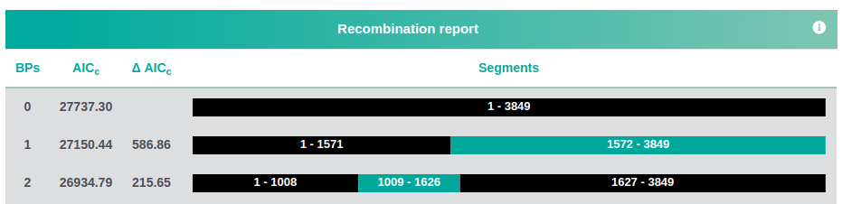
and a map of possible recombination hotspots:

A selection analysis summary and tree (COVID-19 isolate is MN988668_1)

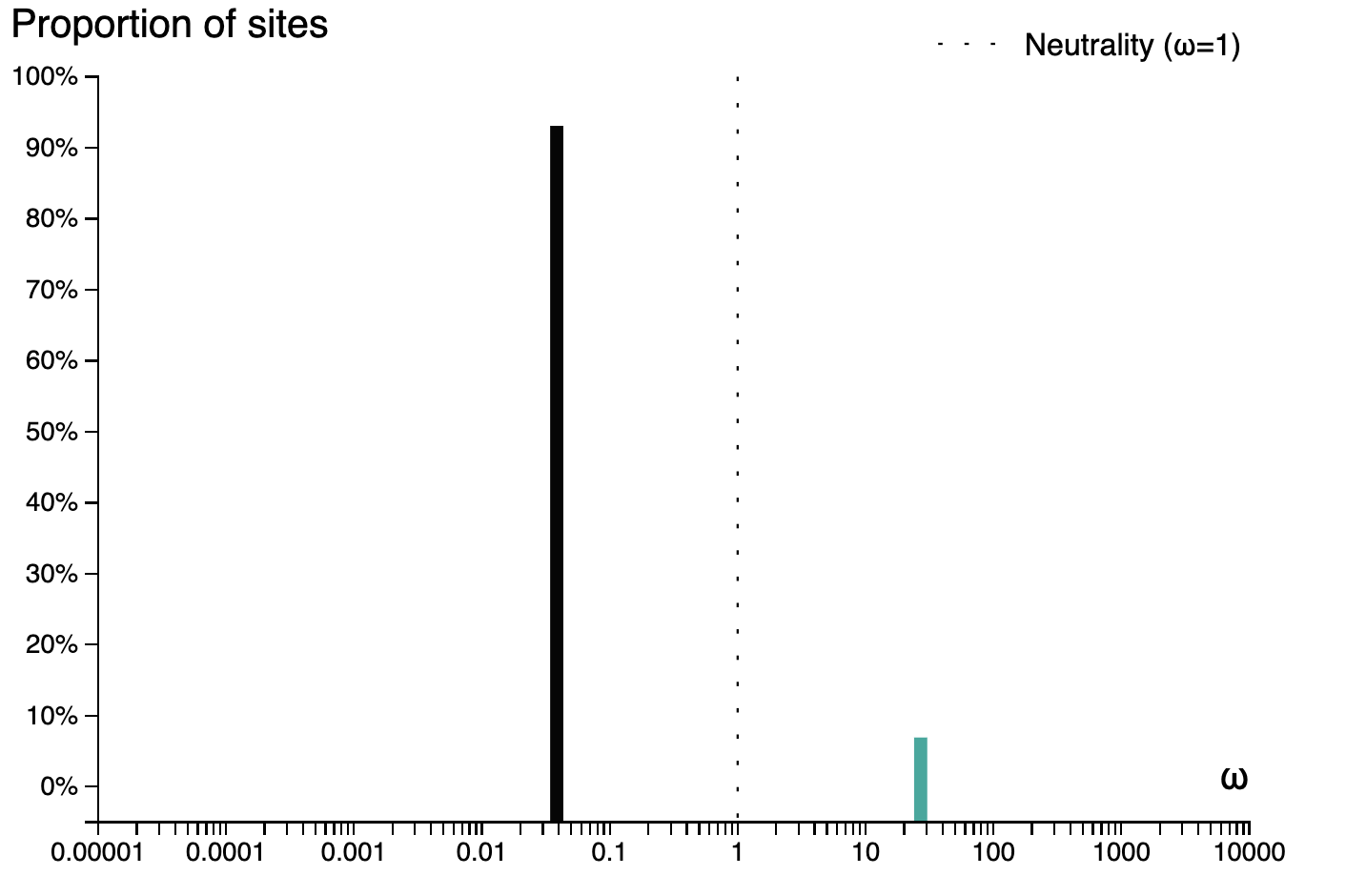
and a plot of the inferred ω distribution for the MN988668_1 branch.

# History and workflow

A Galaxy workspace (history) containing the most current analysis can be imported from here (opens new window).

The publicly accessible workflow (opens new window) can be downloaded and installed on any Galaxy instance. It contains version information for all tools used in this analysis.

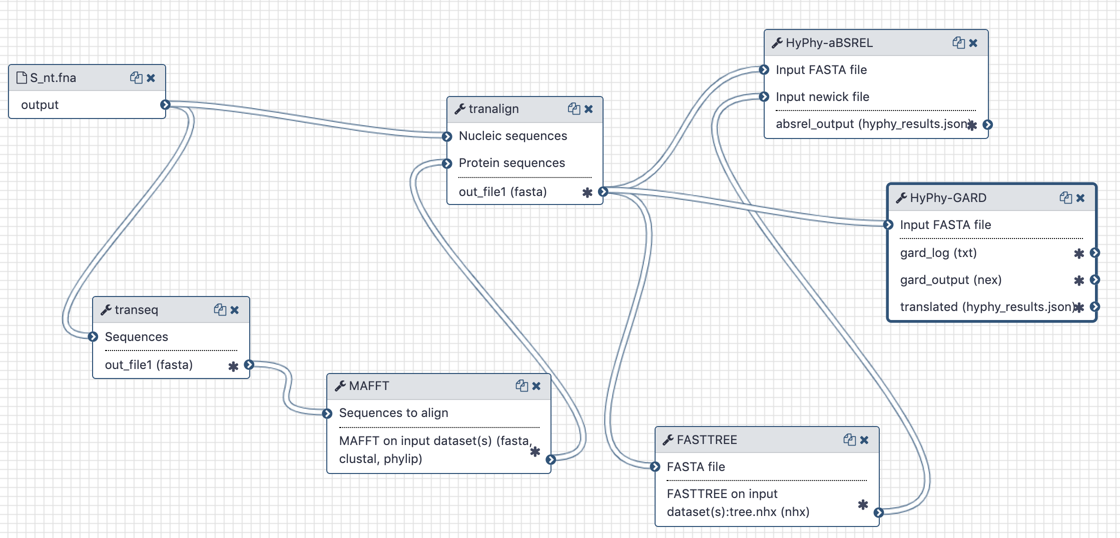
The workflow takes unaligned CDS sequences, translates them with EMBOSS:tanseq, aligns translations using mafft, realigns original CDS input using the mafft alignment as a guide and sends this codon-based alignment to gard.

# BioConda

Tools used in this analysis are also available from BioConda:

Name	Link
`emboss`	(opens new window)
`mafft`	(opens new window)
`hyphy`	(opens new window)
`fasttree`	(opens new window)

# Deploy

# Evolutionary Analysis

# Live Resources

usegalaxy.org	usegalaxy.eu	usegalaxy.org.au	usegalaxy.be	usegalaxy.fr

# What's the point?

# Outline

We then generate a codon-based alignment using the workflow shown below and perform the recombination analysis using the gard tool from the hyphy package.

# Inputs

A set of unaligned CDS sequences for the S-gene.

# Outputs

A recombination report:

and a map of possible recombination hotspots:

A selection analysis summary and tree (COVID-19 isolate is MN988668_1)

and a plot of the inferred ω distribution for the MN988668_1 branch.

# History and workflow

A Galaxy workspace (history) containing the most current analysis can be imported from here (opens new window).

The publicly accessible workflow (opens new window) can be downloaded and installed on any Galaxy instance. It contains version information for all tools used in this analysis.